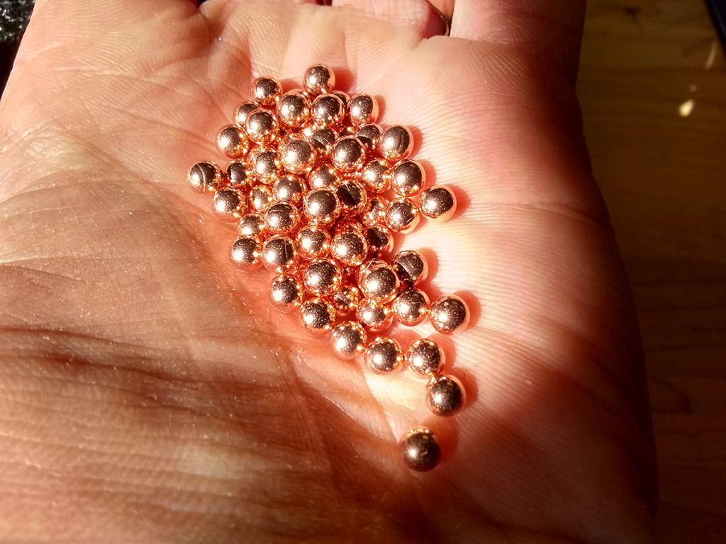
Copper-coated steel BBs, used in several different labs throughout physics and astronomy. Like many of the odds and ends we use for labs and demonstrations, these aren’t used as intended by the manufacturer. In this case, one can only imagine that off-label use is actually safer.
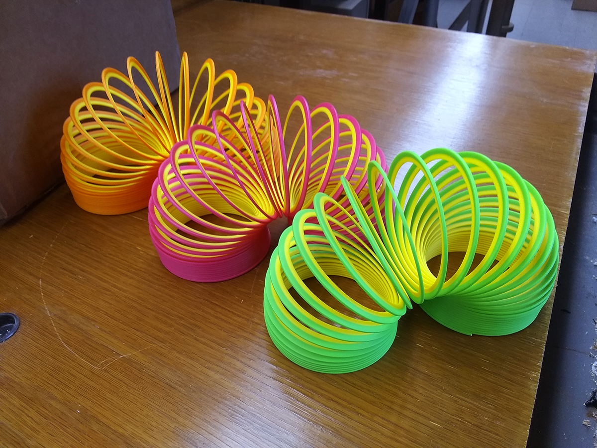
Around here, we get great mileage out of springs, especially when studying waves and oscillations. And few helical coils grab attention quite like a neon-bright Slinky.
Honestly, if you had the choice between eye-searingly bright colors and boring old steel? We hope you’d go for bonus entertainment value, too.
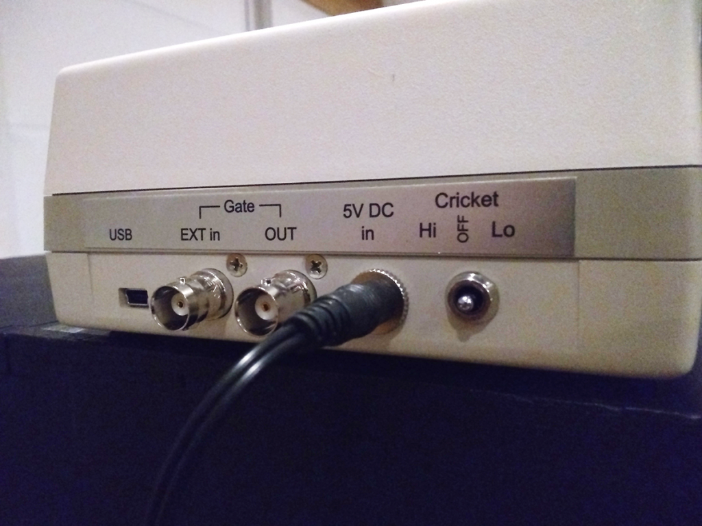
Behold: a box which counts! That’s it, for the most part. It counts pulses of positive voltage. Very quickly, and you can set some thresholds to tell it to count certain values but not others.
It also gates over an interval you set, so you can tell how many pulses it receives over, say, one second. It counts, displays the total, then counts again. Displays the new number.
We use these for our wave/particle duality lab experiment, which relies on counting individual photons. Yes, those. The teeny, massless quantum packets of energy, the messenger particles of electromagnetism. Light. It acts in non-intuitive ways, and the students who think “that’s amazing and I want more!” sometimes become Physics majors.
Part of using this box – just one aspect – is helping convince those students that only one photon at a time can be reaching the photomultiplier tube sensor. At the speed they move, a mind-boggling number of photons can zip through that meter-long box without bunching up. c in air isn’t all that far from c in a vacuum, so if your one-second counts aren’t remotely near 299,792,458 (adjusted for PMT sensitivity and other losses), you know some of those photons are pretty lonesome. Sometimes you need a little math to make sense of things you can’t directly sense.
Crickets.
One other fun aspect is a little switch hidden on the back: cricket. It’s the volume switch, letting the box emit a little beep for every pulse it counts.
If you’re counting pulses from a radioactive source, which arrive randomly, it can be informative to hear these irregular signals, gated and grouped into numbers which show a decaying curve.
If you’re counting 100,000 photons every second, in a room of other lab benches also counting thousands of photons? Less informative, more irritating.
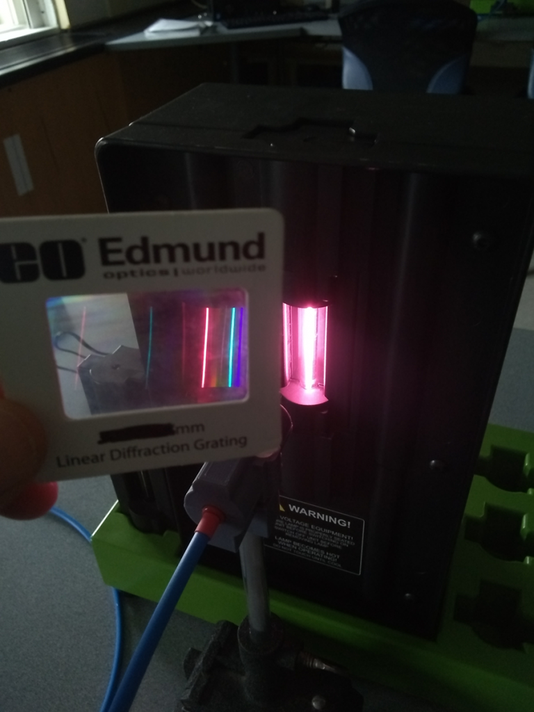
Sometimes, we have old equipment which is rarely, if ever used. Case in point: the mid-20th-century spectroscopes which have been supplanted by digital spectrometers. They’re both effective tools for examining a spectrum of light, one by eye and the other fed by a USB cable. Using a diffraction grating, they split light into its constituent spectrum – its rainbow, more or less – and can identify the presence of individual wavelengths. Not something our eyes can do, as they blend everything together, though that’s very helpful in most situations, such as reading this on your screen.
Summing bands of reddish, greenish, and bluish into a broad rainbow of colors is one neat-o trick.
With a diffraction grating, reflection grating, or prism, you can refract light out along a range of angles which correspond to its constituent wavelengths. Put a sensor at a known angle – your eye or a semiconductor exhibiting the photoelectric effect – and you know the wavelength if you sense a photon. It’s a simple piece of information which can be used to unlock a staggering amount of interesting, related information about what you’re observing.
Hydrogen.
You can also use a diffraction grating to get a quick sense of the entire visible spectrum of a source by holding it off to the side. Remember: the angle of the light’s path change as it refracts, so you’re trying to angle it back to your eye. Hydrogen has a distinctly pinkish-purplish hue when excited at high voltage, and you can see the dominant red and blue lines in its spectrum. With just that one electron to absorb energy and emit photons, the spectrum can only be so complicated.
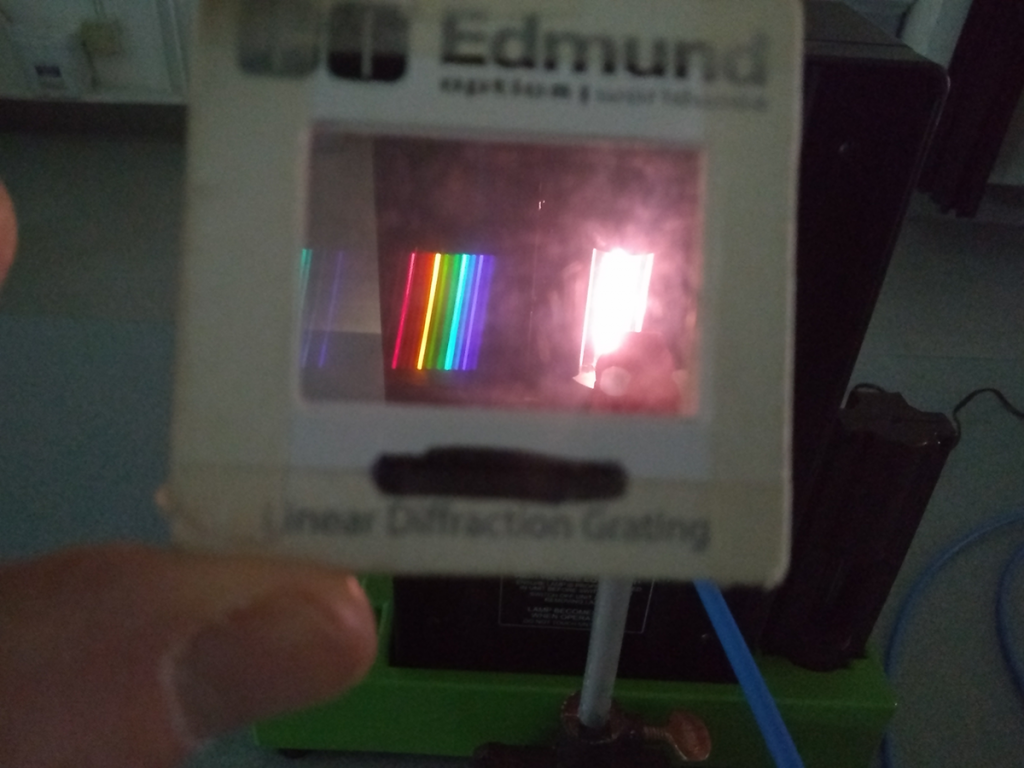
Helium.
That’s in contrast to helium, with its two electrons. The spectrum doesn’t look white, per se, but is much more filled out than hydrogen. Look at those spectral lines, and there are so many more! They’re distinct, measurable, and provide a “fingerprint” that can be immensely useful for scientific study. Or for just looking cool.
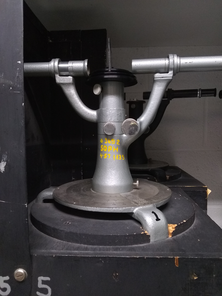
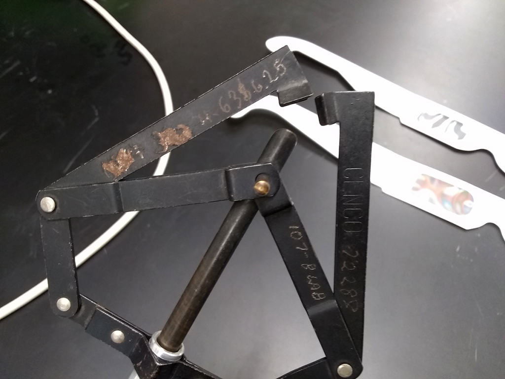
Our old iron optics rails get very little use anymore, as we phase them and their accessories out. Most of them, that is.
We may not use the old glass lenses much – sometimes, not often – but the spring-loaded holders still come out from time to time. They grip certain oddly-shaped objects well, and their heavy iron bases do an excellent job of keeping things like fiber optic cables upright and in place.
Rapidly approaching 60 years old, lens holder. April 1963, $6.25. That’s $61.31 in today’s dollars.
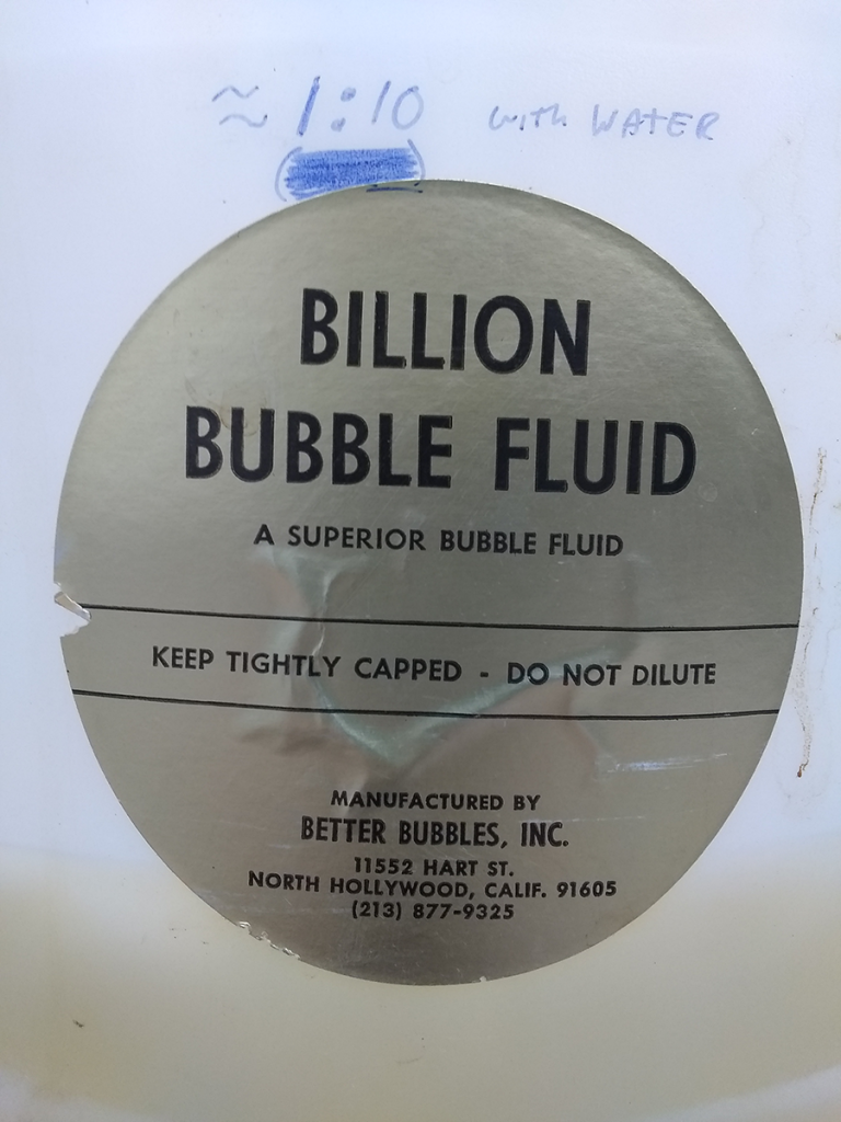
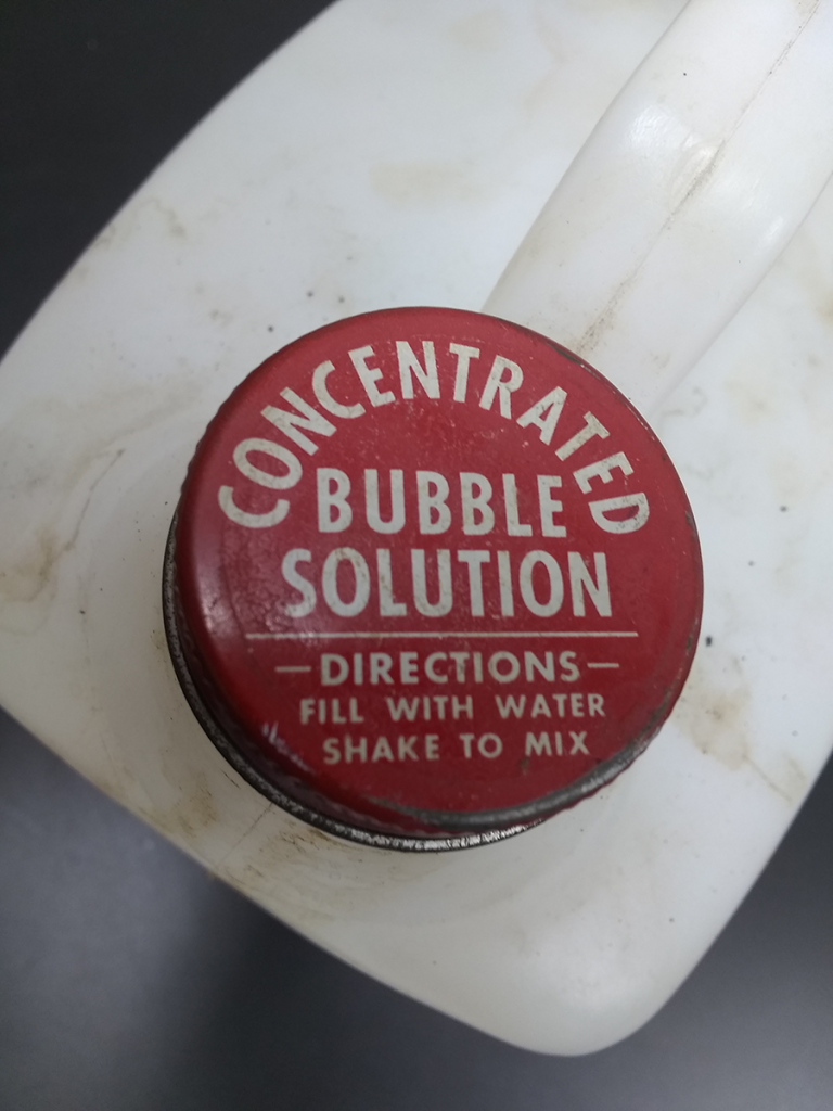
Do you need some superior bubbles? If you’re in the time window between 1961 and 1991, Better Bubbles, Inc. of North Hollywood, Calif., has got you covered. Or, if you’re like us, and you happen to have some of this stuff still around.
Better Bubbles went out of business 32 years ago, so once we’re out of this fluid, we’re out. It is, to be honest, quite superior to the usual soap bubble liquid for kids, at least as far as creating durable thin-film interference patterns. We work diligently to minimize any actual bubbles.
Of special note: the directions for use. The label says “Do Not Dilute,” which seems an odd choice as this stuff flows like thickened liquid dish soap on an icy morning. The lid asks not only for dilution, but actual shaking, which can only result in a I Love Lucy-esque eruption of unending soap bubbles. A hand-written note – clearly the tested and preferred method, and the one still in use – calls for approximately 1 : 10 dilution (vigorously underlined!) with water.
50mL per year, diluted, gently stirred, and the remainder saved for the future. Good luck, whoever needs to find a replacement. Superior bubble fluid is rare stuff.
THIS is how to make a billion bubbles. Do not do this.
There’s a funny thing about important scientific discoveries. The effort and time and careful data collection and building atop previous understandings and innovations and everything else is daunting, difficult, and a massive undertaking. Critical details and a fine understanding may take months, years, or entire careers. A general grasp, though?
Sometimes, you can explain the gist of things with stuff that’s just lying around.
Hubble’s Law, also known as the Hubble-Lemaître Law, describes the expansion of the universe. Galaxies are moving away from ours, and the further away they are, the faster they’re moving. Getting there relied on the Friedmann equations – themselves built upon Einstein’s general relativity – plus Slipher’s redshift measurements of distant galaxies, plus the debates between Shapley and Curtis, plus an understanding of the relationship between luminosity and period in the pulsations of Cepheid variable stars. (They’re like the drinking bird toys of stars.) Plus more, and more, but you get it. A lot goes into explaining the expansion of the universe when all you’ve got is a telescope and spectrometer.
Hubble ran into a real hiccup here. If everything in the universe is moving away from us, and we can correlate the distance and speed in any direction, doesn’t that imply that we’re at the center of the universe? Turns out, no. We’re not.
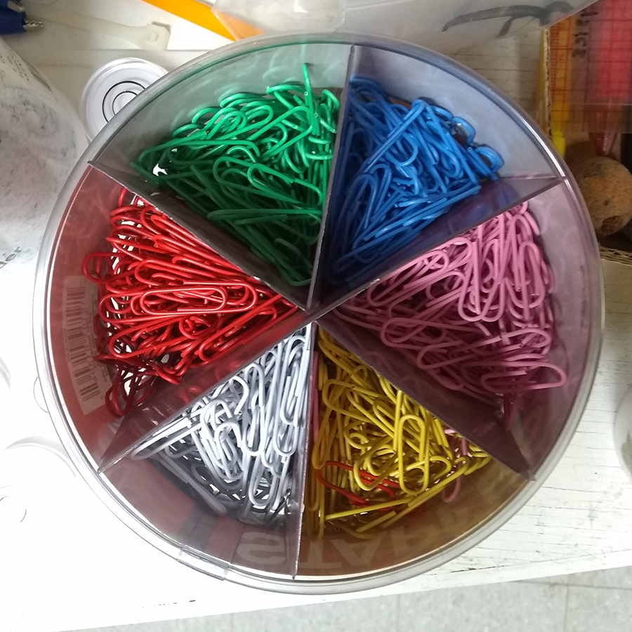
And you can illustrate the principle with a Slinky, a ruler, and some paper clips.
Does the mass of a simple pendulum affect its period of oscillation? The small-angle formula doesn’t include mass, just the length from the pivot to the center of mass and g, the gravitational constant. It’s an approximation that’s pretty good for angles up to 15-20°, and after that it’s into introductory differential equations. Which still don’t use the mass, as it cancels out when applying Newtonian mechanics.
That, however, is for an ideal pendulum, with a massless string and point mass bob in a system without friction and other losses. We’re all out of massless string at the moment, and those point masses are proving elusive. And as neat as it might be to swing a pendulum in a vacuum, the setup sounds like a real challenge.
On top of that, it’s an interesting question that’s really addressing a student’s understanding of measurement and uncertainty. Equations and models illustrate principles, and sometimes do an excellent job of making sense of the world. It’s just that the real world is messier, and wading into that mess – even a little bit – can be enlightening.
Two new pendulum masses, machined to the same dimensions, or close enough that you won’t notice without accurate calipers. Threaded to screw on and off. Aluminum (2.7 g/cm³), checking in slightly under 50 grams each. Brass (8.7 g/cm³), a little over three times the mass, a shade above 150 grams apiece. If we can work with the material, we could make more from anything available.
Lightweight plastics, like Delrin acetal (1.4 g/cm³)? Sure. Denser stuff, like lead (11.3 g/cm³)? Not impossible, but okay, well, no. Even denser? Tungsten, gold, and depleted uranium are all in the 19 g/cm³ range. McMaster-Carr has a range of tungsten alloy rods in stock! (For a small fortune.)
For now, though, it’s two masses, a string, and a stopwatch. Real physics in action.
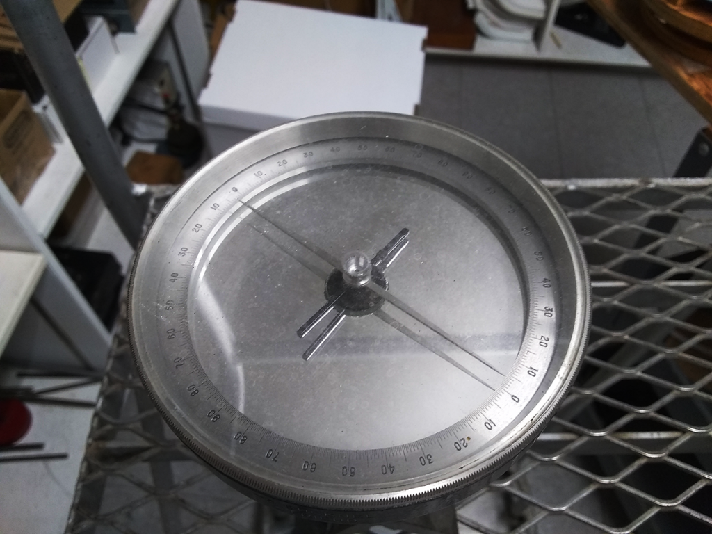
We have many, many compasses scattered about the department. The vast majority come and go as part of the toy kits for PHYS 212, tiny ones useful for illustrating the effects of magnetic fields. Probably more that than for wilderness orienteering. Note: a physics toy kit, despite its educational and entertainment value, is probably insufficient on its own for wilderness survival. Check with the fine folks at Outdoor Education & Leadership for that.
One of the entertaining compass demos is to array a circle of them around an unshielded wire, and seeing the effect of turning the current on and off. Half a dozen little red arrows snapping to attention never loses its neat-o quality.
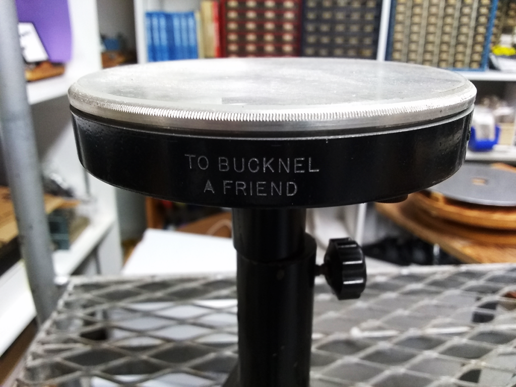
There’s also this little gem, tucked away in one of our closets. Inscribed with a nice little dedication, reading “TO BUCKNEL / A FRIEND” on the side. Which, the longer you look at it, seems a little less clear each time.
Oh. Okay?
Maybe you had to be there? Interpret it as you will.
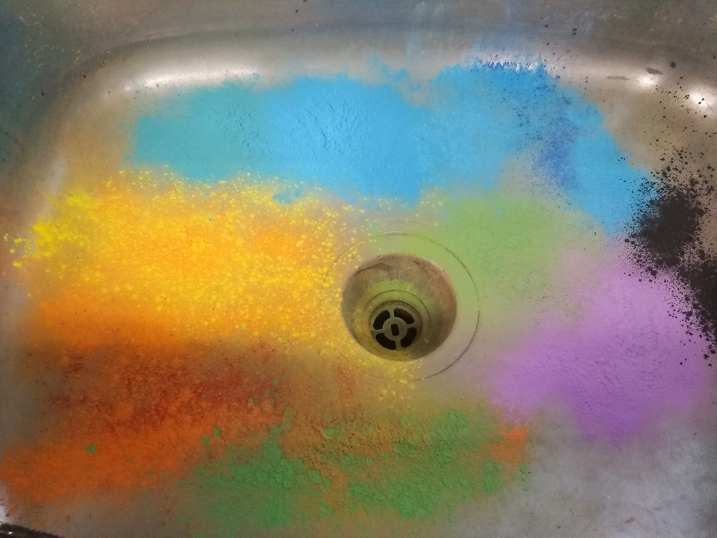
When astronomers study objects they can’t reach, they’re typically limited to visual clues to glean information. Sometimes that’s color variation, like when the ejecta from a crater redistribute layers of rock and soil. Laid down at different times, and made of different materials, the dark and light rings and patches can provide a great deal of insight into how and when a lunar crater formed, for example.
The moon is somewhat less vividly colored than a sink full of tempera paint powder, of course. Electroshock hues make the distinctions easier for the students. We have black, brown, and white in the mix. They work just as well, but never elicit the excited reaction of a brilliant orange or a neon-level magenta.
Intended for mixing your own paint, these are effectively the same as the bright, thick paints in nearly every kids’ art classroom you’ve ever seen. Combined with the play sand, the whole lab starts to smell a little bit like a fun day at preschool.
The aftermath.
In the end, it all becomes a smeared, brownish-gray mix of sand, pigment, and the occasional lost marble or ball bearing. That and a room where every horizontal surface has a new layer of fine, fine dust…